Introduction

The quickest way to get an overview of the evoart process is to watch this video below in which I’m trying to sell you it since the pitch embeds an animated description of the process.

Once you have watched this, please read the article below to get a more in-depth understanding.

It begins with pixels

A pixel is a rectangular area of color and is the smallest area of color that a computer monitor can display. Digital images are made up of thousands, sometimes millions, of pixels arranged in a 2D plane. Pixels are very small and so when the image is displayed on a computer monitor we do not normally see the individual pixels. In the image below, a digital picture has been magnified and a grid placed over the top. Each grid square contains a single pixel of the original image.

Each pixel is a block of solid color. The color of a pixel can be represented in a number of ways. From our perspective these are all equivalent and can be reduced to the canonical Red-Green-Blue mixture representation. Now consider that each pixel can be referenced via its x and y coordinates. In digital images the point of reference is usually taken as the upper left, so that the x coordinate increases left-to-right and the y coordinate increases top-to-bottom. Using this idea, the image below shows a 4x4 square of “pixels” with their x and y coordinates written in the form (y,x).

Now we know that the color of a pixel is determined by its red, green, and blue components and that we can assign coordinates to pixels. The core concept behind evolving images (using the methodology I did), is that we can generate pictures by making the red, green, and blue color components of each pixel, a function of its coordinates. That is, the color of each pixel is a function of its position. Aesthetic evolution is nothing other than the “breeding” of the underlying functions of the “most pretty” images for thousands of generations, in a way analogous to the selective breeding of livestock.

Images from functions

As mentioned in the introduction, images can be generated from functions; a function which returns a color and which takes as arguments a pair of coordinates, is evaluated for each position in the image to generate the pixel colors for an entire image.

As an illustrative example, consider the function which returns the following color (expressed in terms of its red, green, and blue components which each assume a value between 0 and 1)

$$ red;component = x $$

$$ green;component = 0 $$

$$ blue;component = 0 $$

This function keeps the green and blue components of each pixel constant at zero, whilst increasing the red component with x. Evaluating this function for a 250x250 pixel image results in the following image:

In expectation with the function definition, pixel redness gradually increases across the image from left to right.

Note that the x value starts at zero on the far left, and we define it to end having value one at the far right. The value that x is increased as we move to the right, therefore depends on how big the image is, but this is easy to calculate on a computer.

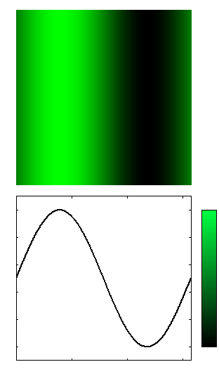
As another example consider the following function

$$ red;component = 0 $$

$$ green;component = \frac{1}{2} \cdot (1 + \sin x) $$

$$ blue;component = 0 $$

The figure below shows the generated image, and the associated function. A color bar is included next to the plotted function to illustrate the correspondance of function values with colors.

Functions as trees

Mathematical functions can be expressed as mathematical trees. Consider the function $$ f(x) = (x+3)*x $$. In tree form, this looks like

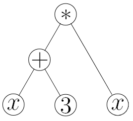
In computer science, like everything else, trees are upside-down. The nodes at the bottom are called leaves and the node at the top is called the root.

The function is evaluated starting at the leaves. The values of the leaves are passed to the function at the node above them to get new values, which are then passed up to the function above them, on so on until the root node is evaluated and the tree returns a value.

Thus in the example above, $$ x $$ and $$ 3 $$ are passed to the function $$ + $$ which computes $$ (x+3) $$, this is passed along with the right-most leaf $$ x $$ to the function $$ * $$ which computes the result of the tree $$ (x+3)*x $$.

By randomly choosing function nodes and at what point to place leaves, we can “grow” function trees.

The root of a function-tree which represents an image is a function which returns a pixel color and has 3 branches, one for each of the color components red, green, and blue. Lets call the root function $$ rgb $$, it will take 3 arguments, the amount of red, green, and blue. Imagining that when evaluated it will return a color, the function-tree for the pixel-color function looks abstractly like this

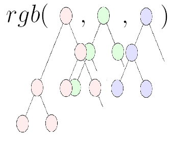
where the function $$ rgb $$ takes 3 values as input, one for each color component red, green, and blue. The picture illustrates the fact that each color is a separate subtree. Each subtree is some function which can depend on the pixel coordinates. Evaluating the $$ rgb $$ function for each coordinate in a plane generates an image as discussed in the last section.

Mutating and breeding function trees

In order to “breed” the most pretty pictures, we make their underlying functions undergo analogues of sexual and asexual reproduction.

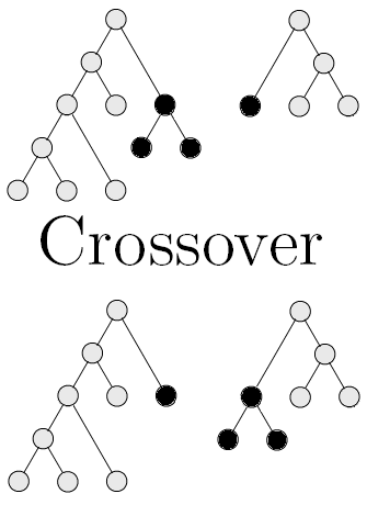
Sexual reproduction is simulated by what is called crossover: given two function-trees a subtree from each is selected at random and then the subtrees are swapped. This is illustrated below:

Asexual reproduction is simulated by what is called mutation: given a function-tree, a node is selected at random. If it is a function node, then we replace the function with a random function taking the same arguments, and if it is a leaf then we replace the leaf with either a new random leaf or we can even grow a new subtree at that point. This is illustrated below:

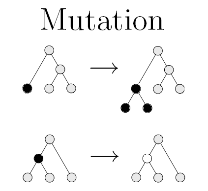
Two forms of mutation are shown, in the first form, a leaf is replaced by a new subtree, and in the second a function node is changed to another function.

These are very simple ways to modify existing function-trees to produce “offspring”. By using our imagination, ways different to and many variants of the above sexual and asexual reproduction methods can be conceived to produce a wide variety of offspring.

Evolving images

We have seen previously three important things:

1. Pictures can be generated from functions
2. Functions can be represented as trees
3. Trees can be “bred” together or mutated to produce new trees

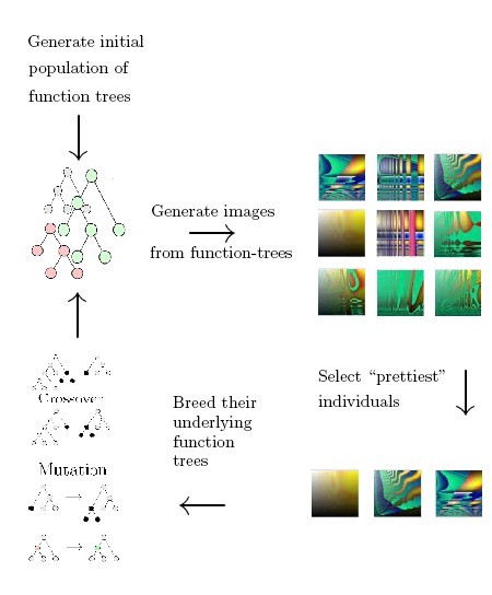
With this information under our belt it will be easy to comprehend how the evolution of images works. Algorithmically we do the following

1. Generate an initial population of random-function trees
2. Generate their corresponding pictures
3. Select the best looking pictures from the current generation
4. Breed the underlying function trees of those selected
5. The offspring become the new generation of pictures
6. Goto 2

Thus we see that the evolution of images proceeds by repeatedly selecting and breeding the best looking pictures. After many hundreds of generations the images gradually improve and become more and more interesting as the underlying genetic forms (function-trees) are evolved.

The process of aesthetic evolution is illustrated below:

In practice the above procedure is executed in a more flexible way; typically one maintains several repositories of good evolved images which can be bought into the current generation at any time. This allows, for example, images from separate runs of the above procedure to be bought together for breeding. One can imagine many branches of image histories which can be recombined at will. By being flexible we enable ourselves to generate amazing pictures.

Now that you understand the basics behind evolving images. Click here to take a look at the results.

Appendix: More complex images and their functions

It is illustrative to examine the underlying functions for a few complicated images, so that one can understand the complexity leap involved. Some examples are presented in this section.

The image below is relatively simple, being comprised of only 49 nodes and a tree depth of 14:

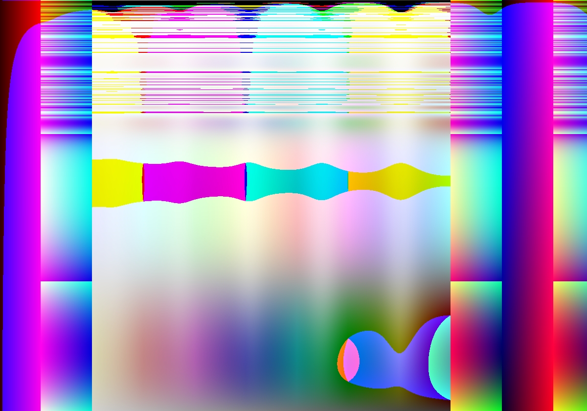
This is the function that generates it:

HSV_to_RGB( new_hsv( ( ( float) add( 7,neg( sub( complex_degrees_to_radians( divide( x,5) ) ,broken_log( tan( -8) ) ) ) ) ) ,( ( float) sin( divide( ( ( int) 8.066796) ,sin( divide( broken_log( M_E) ,y) ) ) ) ) ,( ( float) sin( divide( divide( ( ( float) x) ,divide( ( ( float) exp( divide( ( ( float) x) ,divide( ( ( float) exp( sin( complex_degrees_to_radians( sin( x) ) ) ) ) ,sub( ( ( int) 1.000000) ,y) ) ) ) ) ,y) ) ,cos( ( ( 0) ?complex_radians_to_degrees( x) :mul( ( ( float) 1.000000) ,complex_radians_to_degrees( exp( 5) ) ) ) ) ) ) ) ) )

The image below is much more complicated. It has 249 nodes and a tree depth of 24:

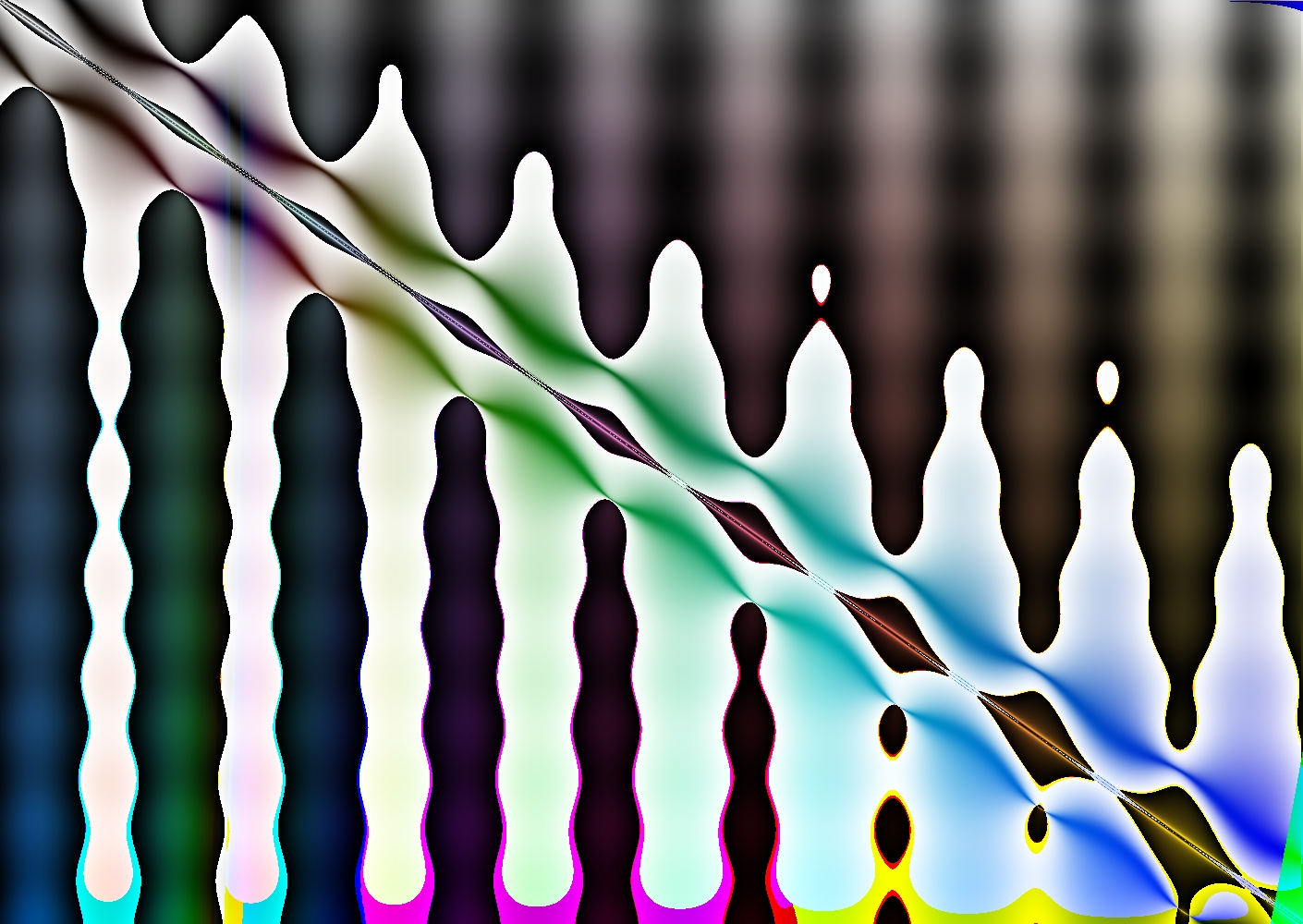
Here is the function that generates it:

HSV_to_RGB( new_hsv( ( ( float) protected_log( sub( ( ( int) complex_modulus_squared( complex_scalar_mul( complex_conjugate( complex_sub( complex_sub( complex_sub( complex_new( sub( 8,7.525226) ,-4.687266) ,complex_mul( complex_new( -9.054818,6.145719) ,complex_new( y,( ( int) 1.306550) ) ) ) ,complex_new( add( protected_log( y) ,tan( complex_argument( complex_new( 8.440938,-8.329001) ) ) ) ,floor( -2.278851) ) ) ,complex_conjugate( complex_new( -5.820303,3.686237) ) ) ) ,add( ( ( int) x) ,x) ) ) ) ,ceil( ( ( float) complex_argument_degrees( complex_new( 4.481138,2.879883) ) ) ) ) ) ) ,( ( float) y) ,( ( float) sin( complex_argument_rad_proper( complex_scalar_div_protected( complex_div_protected( complex_div_protected( complex_add( complex_rotate( complex_new( mul( x,1.076204) ,x) ,exp( ( ( int) 4.916573) ) ) ,complex_new( 3.168356,9.608354) ) ,complex_new( -9.892548,8.779981) ) ,complex_sub( complex_add( complex_add( complex_sub( complex_rotate( complex_new( 5.570485,3.863986) ,broken_log( x) ) ,complex_sub( complex_conjugate( complex_mul( complex_mul( complex_rotate( complex_new( 8.518827,9.531490) ,protected_log( sub( x,y) ) ) ,complex_div_protected( complex_new( 8.454529,-3.901050) ,complex_new( 3.977127,9.449823) ) ) ,complex_rotate( complex_new( -1.896125,7.405597) ,neg( y) ) ) ) ,complex_new( -9.425669,7.165792) ) ) ,complex_rotate( complex_rotate( complex_add( complex_add( complex_rotate( complex_new( -7.817081,-6.535177) ,complex_degrees_to_radians( y) ) ,complex_div_protected( complex_new( -7.477049,1.884666) ,complex_new( -1.634072,0.823157) ) ) ,complex_new( 1.730793,-3.415812) ) ,( ( int) cos( broken_log( add( pow( x,sub( ( ( float) mul( protected_log( exp( neg( complex_modulus_squared( complex_add( complex_scalar_mul( complex_new( 0.800652,-2.480108) ,0) ,complex_new( 7.072666,2.538549) ) ) ) ) ) ,exp( complex_argument_rad_proper( complex_sub( complex_new( -2.912281,-9.784648) ,complex_new( -6.592574,-3.081946) ) ) ) ) ) ,2) ) ,x) ) ) ) ) ,( ( int) x) ) ) ,complex_rotate( complex_sub( complex_new( -2.855067,5.798346) ,complex_div_protected( complex_add( complex_new( -8.069270,2.494037) ,complex_sub( complex_mul( complex_sub( complex_new( -7.798228,4.766676) ,complex_new( -3.213019,7.679907) ) ,complex_new( -4.252113,1.289872) ) ,complex_add( complex_conjugate( complex_scalar_div_protected( complex_add( complex_rotate( complex_new( 1.801271,-3.462400) ,x) ,complex_conjugate( complex_new( 1.550093,-4.248504) ) ) ,protected_log( complex_argument_rad_proper( complex_new( 5.205422,-8.070377) ) ) ) ) ,complex_new( -3.789560,2.683181) ) ) ) ,complex_rotate( complex_new( 0,cos( pow( exp( 1) ,( ( boolean_is_less_than_or_equal_double( neg( ( ( int) 7.796022) ) ,divide( 1.812069,y) ) ) ?( ( boolean_is_less_than( y,3.427348) ) ?floor( y) :sin( x) ) :complex_argument_degrees( complex_scalar_mul( complex_new( -1.438167,0.839113) ,( ( int) 0.820962) ) ) ) ) ) ) ,complex_degrees_to_radians( x) ) ) ) ,( ( int) 5.561037) ) ) ,complex_new( 2.551302,8.219454) ) ) ,( ( float) floor( divide( -8.000000,complex_argument_rad_proper( complex_sub( complex_rotate( complex_new( ( ( float) mul( y,mul( pow( complex_modulus( complex_new( -5.770987,-1.758157) ) ,complex_modulus( complex_new( 8.194765,-7.392895) ) ) ,( ( boolean_is_less_than( x,x) ) ?complex_modulus( complex_new( 5.993767,1.768086) ) :complex_modulus_squared( complex_new( 9.645488,6.740700) ) ) ) ) ) ,complex_modulus_squared( complex_rotate( complex_div_protected( complex_scalar_mul( complex_new( -2.981901,5.089888) ,broken_log( complex_modulus( complex_new( -0.943985,-8.788256) ) ) ) ,complex_new( -9.845440,9.606460) ) ,complex_argument_rad_proper( complex_div_protected( complex_new( 9.620297,3.106028) ,complex_conjugate( complex_new( -9.417724,exp( pow( ( ( int) 1.237943) ,complex_modulus_squared( complex_new( 7.933170,6.635299) ) ) ) ) ) ) ) ) ) ) ,y) ,complex_scalar_mul( complex_add( complex_mul( complex_mul( complex_new( -4.999893,5.324683) ,complex_new( 4.187125,9.156792) ) ,complex_div_protected( complex_new( -0.399050,-1.186179) ,complex_sub( complex_scalar_mul( complex_new( 8.790867,6.072102) ,add( x,y) ) ,complex_div_protected( complex_mul( complex_new( 9.514227,-6.065766) ,complex_new( -8.530125,-3.344384) ) ,complex_mul( complex_new( 7.137485,4.353529) ,complex_mul( complex_new( 1.571602,3.818364) ,complex_scalar_div_protected( complex_new( 4.454805,-4.306024) ,complex_modulus( complex_new( 4.582274,8.375720) ) ) ) ) ) ) ) ) ,complex_div_protected( complex_mul( complex_new( -0.418429,-6.460651) ,complex_new( -6.712513,-5.919816) ) ,complex_mul( complex_new( 0.751718,-9.902483) ,complex_new( -6.125777,-3.839288) ) ) ) ,y) ) ) ) ) ) ) ) ) ) ) )